


Friends, Microsoft Excel is used in every field nowadays. Be it a business or a school project, there is always a need for Microsoft Excel. But its formulas make your Microsoft Excel work even easier. In today’s article we will discuss some Excel Formulas in Hindi You will see which will prove to be very useful in your Excel work.
If you use the right formula at the right place, you can save a lot of time and effort. Read this article carefully till the end.
Excel Formulas in Hindi
Actually, there are many such formulas of Microsoft Excel which you can adopt. But we will know about some major formulas about which you must know. We will also learn one by one how you can use these formulas.
1: SUM formula
Sum formula is used to add the numbers given in any cell in Excel. This is a basic formula of Excel with the help of which you can add two or more numbers.
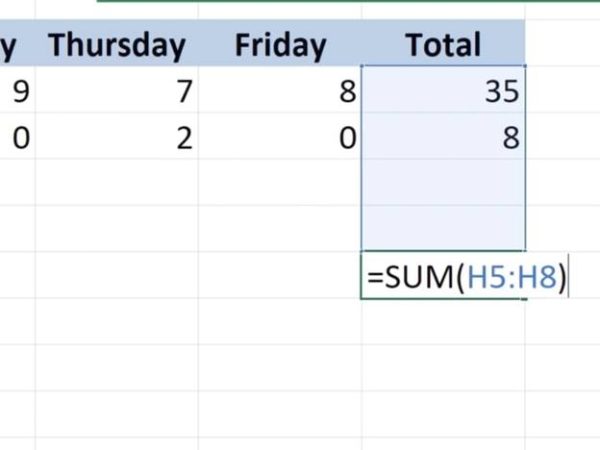
Formula: =SUM(H5:H8)
Here, by applying the formula =SUM(H5:H8) all the numbers will be added, 35+8 i.e. the result will be 43.
2: Product formula
Product formula is also one of the basic formulas, using this formula you can multiply two or more cells.
Formula: =PRODUCT(A3:A5,B3:B5)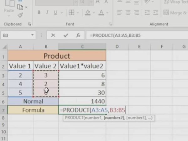
The formula =PRODUCT(A3:A5,B3:B5) has been applied to multiply all the values 2,4,5,3,2,and 6 on the sheet shown above, after which the result will be 1440.
3: Power formula
The POWER formula is used to multiply the number in any cell by the same number repeatedly. Using this formula, square, cube, etc. of numbers can be calculated.
Formula : =POWER(C4,D4)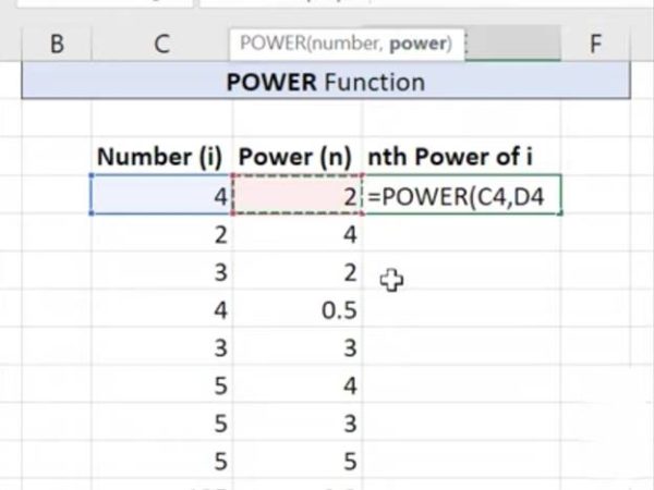
On applying the power formula on cell E4, the power of 4 will be 2 and the result will be 16.
4: MAX formula
The MAX formula is used to find the largest number among all the cells in Excel. The MAX formula can be used in both rows and columns.
Formula: =MAX(E2:E22)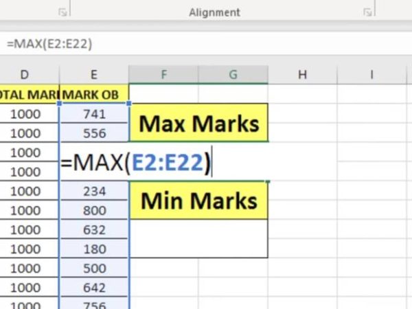
By applying Max formula on the cell shown above, the largest number i.e. 800 results will be seen.
5: MIN formula
MIN formula is used to find the smallest number among the numbers present in the Excel sheet.
Formula: =MIN(E2:E22)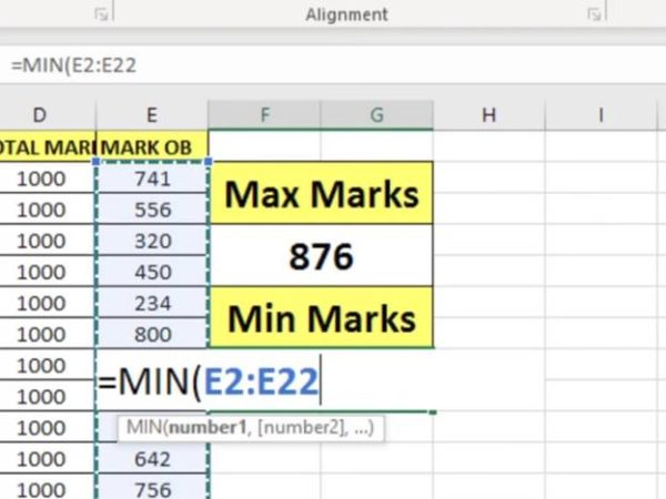
The smallest number can be found using the minimum formula, applying this formula in the list given above, the result will be 234.
6: AVERAGE formula
If you want to find the mean or average of the numbers present on the Excel sheet, then you can use the average formula for this.
Formula: =AVERAGE(C3:C8)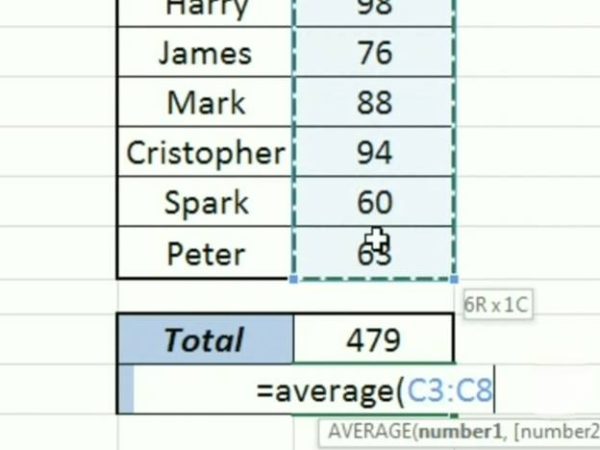
This formula can be used to find the average of the numbers shown above, after which the result will be 30+98+76+88+94+60+63/7 i.e. 68.4285.
7: RANK formula
If you excelIf you want to calculate the rank based on the numbers present on the letter, then you can use the RANK formula. Using the rank formula, you can get the rank on the basis of highest number or lowest number by choosing ascending or descending.
Formula: =RANK(B2, reference)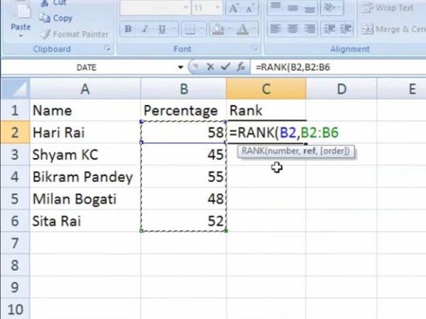
In this formula, instead of the number, you have to select the cell whose rank you want to find. On the reference, you will have to select all the cells with which you want to find the rank of this cell.
The result in cell C2 shown above will be 1, because the number shown in cell B2 is greater than all the other numbers.
8: Count formula
The Count formula can be used to count the cells on an Excel sheet that contain a number.
Formula: =COUNT(L4:L12)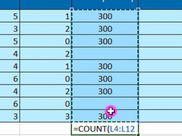
The Count formula is used to count the cells shown above that contain a number. The result of this formula will be 7, this is because numbers have been entered in 7 cells.
9: Countblank formula
If you have a sheet that has some blank cells along with numbers and you want to count those blank cells, then you can use the countblank formula.
Formula : =COUNTBLANK(E76:E84)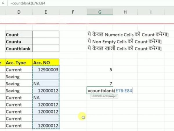
Using the CountBlank formula on the cells shown in the table above will result in 2 because two of the selected cells in the table are blank.
10: CountA formula
CountA formula is a formula with the help of which you can count the cells in which some number or text has been entered. Empty cells are not counted when this formula is used.
Formula: =COUNTA(E76:E84)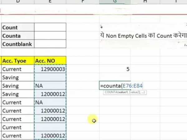
Applying this formula to count all the filled cells in the table shown above will result in 7 in that cell. Using this formula, two empty cells will not be counted.
11: Now formula
If you want to enter the current time and date in any cell on Excel in the format DD/MM/YYYY HR:MM, then you can use the now formula.
Formula: =NOW()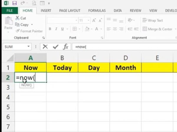
Now formula can be used to show the current date and time, using this formula the result will be something like this – 09/01/2024 14:25
12: Today formula
Many times we have to enter today’s date on Excel, for this TODAY formula can be used. After using this formula, you can enter today’s date in DD/MM/YYYY format.
Formula : =TODAY()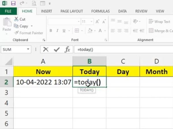
If you want to put today’s date in any cell, then you can use =today() formula, if you use this formula on 09/01/2024, the result will be 09/01/2024.
13: Year formula
If you want to find out the year from the date present in a cell, then you can use the year formula. To use this formula, type the method in the cell: DD/MM/YYYY HR:MM, DD/MM/YYYY or
Must be in MM/YYYY format.
Formula: =YEAR(A1)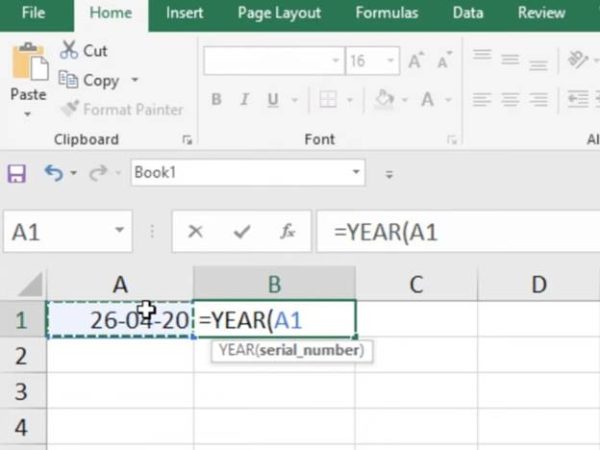
If you want to find out the year from 26-04-2020, then year formula can be used for this. After using this formula the result will be 2020.
14: Month formula
Month formula in Excel is used to extract the month number from the date present in any cell. For this you have to select that cell in the formula, like we have selected cell A3.
Formula: =MONTH(A3)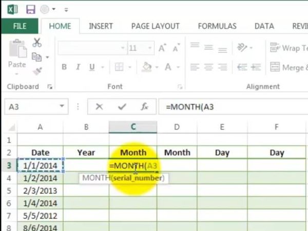
By writing this formula in cell C3, the month can be separated from the date 1/1/2014. Using this formula, the result will be 1 i.e. the first month.
15: Day formula
DAY formula is used to find the day from any date. Using this formula you can find the name of the day like Sunday, Monday, Tuesday, etc.
Formula: =TEXT(D4,”DDDD”)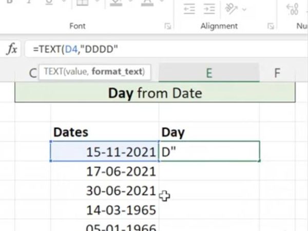
To know which day it was on 15-11-2021, the formula =TEXT(D4,”DDDD”) can be used. On writing this formula, the result on the sale will be Monday, that is, this date was Monday.
16: REPT formula
If you want to repeat any cell present in Excel, then REPT formula can be used for this. In this formula, you can also enter the number of times you want to repeat the text or number present on a cell.
Formula: = REPT(B2, n)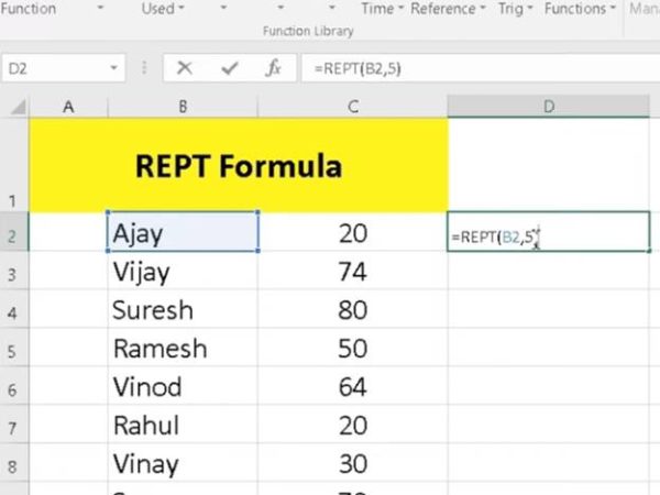
In place of n, you can enter the number of times you want to repeat the text or number written in a cell. For example, if you want to repeat Ajay five times, you can use the formula shown above and write 5 in place of n. In this case the result will be AjayAjayAjayAjayAjay.
17: Trim formula
The TRIM formula is used to remove spaces between numbers or sentences. After using this formula, you can remove more than one space between sentences.
Formula: =TRIM(B143)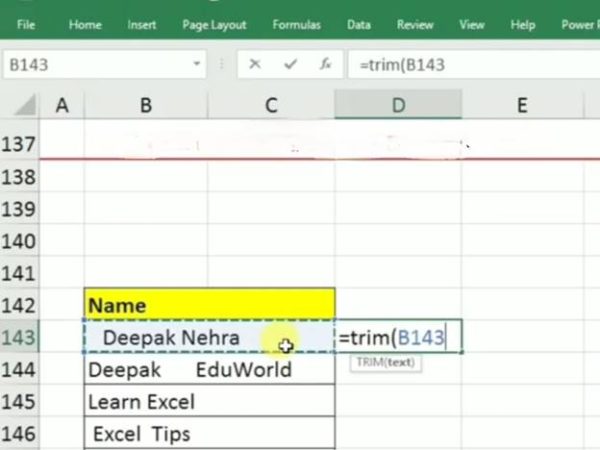
Applying Trim formula on cell B143 in the photo shown above will remove more than one space from the name shown and the result will be Deepak Nehra.
18: MEDIAN formula
Median formula is used in Excel to find the middle number among many numbers.
Formula: =MEDIAN(B2:B8)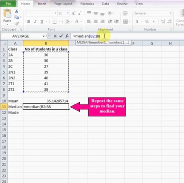
The numbers shown above are 27, 30, 30, 39, 39, 40, 41, applying the median formula on this will give the result 39 on B11 cell.
19: MODE formula
The Mode formula can be used to find the most frequently occurring numbers on an Excel sheet.
Formula: =MODE(C6:G6)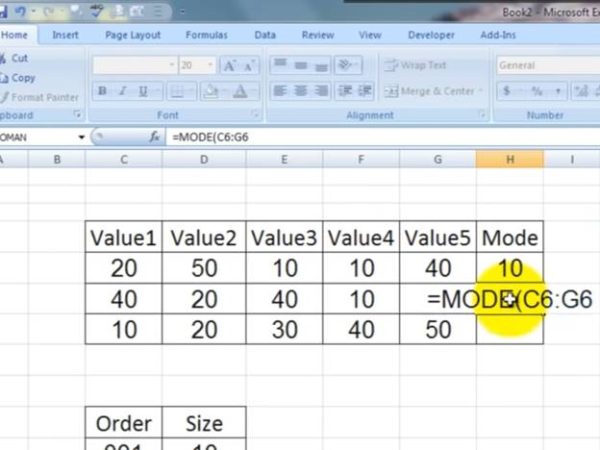
The second column shown above contains the numbers 40, 20, 40 and 10, here 40 is the next highest number.
On applying the mode formula, the mode of these numbers i.e. 40 will be visible.
20: LEFT formula
Left formula is used to write the first few numbers or alphabets from any big number or sentence.
Formula: =LEFT(B209, n)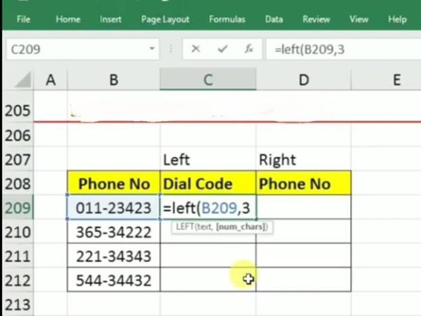
Suppose you want to keep three numbers at the beginning of a number or word, then you can write 3 in place of n.
Using the formula in the cell shown above will result in the number 011. This is because 3 is written in place of n above.